41 pivot table 2 row labels
Excel Pivot Table with nested rows - Basic Excel Tutorial 2. Once you create your pivot table, add all the fields you need to analyze data. How to add the fields. Select the checkbox on each field name you desire in the field section. The selected fields are added to the Row Labels area in the layout section. You can drag a field you want from the field section to an area in the layout section. Combining two+ Columns to form one Row label column in ... Re: Combining two+ Columns to form one Row label column in Pivot Table. Select a cell in your pivot table. Press Alt, then D, then P (i.e. in succession; not all at the same time), to call up the Pivot Table Wizard. Click "
pivot table how to combine 2 row labels | MrExcel Message ... Excel Questions pivot table how to combine 2 row labels sdsurzh Nov 6, 2013 S sdsurzh Board Regular Joined Sep 27, 2009 Messages 248 Nov 6, 2013 #1 Hi, i am having the pivot table in the below format. my concern is how i can combine both A & AA together the source is from data connection and not from the excel.

Pivot table 2 row labels
How to Add Rows to a Pivot Table: 9 Steps (with Pictures) 2 Click any cell in the PivotTable. This opens the PivotTable Fields panel on the right side of Excel. If you have already moved the appropriate field to the Rows area but don't see a row that's in your source data, just press Alt + F5 or right-click the pivot table and select Refresh. 3 Drag a field into the "Rows" area on PivotTable Fields. How to Add Two-Tier Row Labels to the Pivot Table in ... Step 1: Click on any cell in the Pivot Table so that the Pivot table editor sidebar appears on the right side of Google Sheets. Pivot Table, with Pivot table editor sidebar visible. As you can see, the item column is used as the row labels or headers in the Pivot table. Pivot Table adding "2" to value in answer set 1) Right click your pivot table -> Pivot table options -> Data -> Change "Number of items to retain per field" to NONE 2) Wipe all rows in your data source except for the headers 3) Refresh the pivot table 4) Save, and close all instances of Excel 5) Reopen the file, and paste your data 6) Refresh the pivot table
Pivot table 2 row labels. Design the layout and format of a PivotTable Click anywhere in the PivotTable. This displays the PivotTable Tools tab on the ribbon. On the Options tab, in the PivotTable group, click Options. In the PivotTable Options dialog box, click the Layout & Format tab, and then under Layout, select or clear the Merge and center cells with labels check box. Sort multiple row label in pivot table - Microsoft Community Sort multiple row label in pivot table. Hi All. Could anybody suggest how to sort the pivot table row field data if it contains multiple headers :-. for example : In below given example I want to sort the data of column B in asending order , but when I am applying sorting here it is not sorting. Thanks in advance for your suggestion. How to add side by side rows in excel pivot table ... To display more pivot table rows side by side, you need to turn on the Classic PivotTable layout and modify Field settings. For example will be used the following table: You have to right-click on pivot table and choose the PivotTable options. Then swich to Display tab and turn on Classic PivotTable layout: Pivot table row labels side by side - Excel Tutorials You can copy the following table and paste it into your worksheet as Match Destination Formatting. Now, let's create a pivot table ( Insert >> Tables >> Pivot Table) and check all the values in Pivot Table Fields. Fields should look like this. Right-click inside a pivot table and choose PivotTable Options…. Check data as shown on the image below.
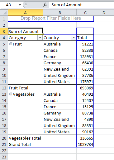
How to rename group or row labels in Excel PivotTable? 1. Click at the PivotTable, then click Analyze tab and go to the Active Field textbox. 2. Now in the Active Field textbox, the active field name is displayed, you can change it in the textbox. You can change other Row Labels name by clicking the relative fields in the PivotTable, then rename it in the Active Field textbox. ExtendOffice - Beste tools voor kantoorproductiviteit ExtendOffice - Beste tools voor kantoorproductiviteit Multi-level Pivot Table in Excel (In Easy Steps) First, insert a pivot table. Next, drag the following fields to the different areas. 1. Category field and Country field to the Rows area. 2. Amount field to the Values area. Below you can find the multi-level pivot table. Multiple Value Fields First, insert a pivot table. Next, drag the following fields to the different areas. 1. get a row label from pivot table - Microsoft Tech Community Alternatively you may work with cube assuming you are at least on Excel 2010, as I remember it's the first which supports data model. Create PivotTable and after that convert it to cube formulas. Now you may take these formulas and convert it to form you need, for example. =CUBEVALUE( "ThisWorkbookDataModel", CUBEMEMBER("ThisWorkbookDataModel ...
Remove PivotTable Duplicate Row Labels [SOLVED] Re: Remove PivotTable Duplicate Row Labels Sometimes when the cells are stored in different formats within the same column in the raw data, they get duplicated. Also, if there is space/s at the beginning or at the end of these fields, when you filter them out they look the same, however, when you plot a Pivot Table, they appear as separate headers. Pivot table - Wikipedia Row labels are used to apply a filter to one or more rows that have to be shown in the pivot table. For instance, if the "Salesperson" field is dragged on this area then the other output table constructed will have values from the column "Salesperson", i.e. , one will have a number of rows equal to the number of "Sales Person". excel - Extract Pivot Table Row Label (not value) - Stack ... In Excel 2010, I have a pivot table, in compact form, with 3 Row Labels (that represent a management hierarchy). Which of the 3 management levels is displayed in a particular row will change from day to day. (The source data is on another spreadsheet with the fields Manager L3, Manager L2 and Manager L1 in columns with John Smith, Gary Glen and ... Pivot Table "Row Labels" Header Frustration - Microsoft ... Public Sector. Internet of Things (IoT) Azure Partner Community. Expand your Azure partner-to-partner network. Microsoft Tech Talks. Bringing IT Pros together through In-Person & Virtual events. MVP Award Program. Find out more about the Microsoft MVP Award Program.
23 things you should know about Excel pivot tables | Exceljet
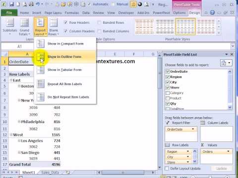
Microsoft Excel - showing field ... - ifonlyidknownthat In Microsoft Excel 2007 and 2010, by default if you create a pivot table, instead of showing the field names, it will say row labels and column labels. Show in Outline Form or Show in Tabular form. The relevant labels will To see the field names instead, click on the Pivot Table Tools Design tab,…

How to Use Excel in 2017: 14 Simple Excel Shortcuts, Tips & Tricks
Change the pivot table "Row Labels" text | MrExcel Message ... Feb 4, 2021. #3. mart37 said: Click on the cell and typ the text. Click to expand... Thanks mart37. So simple! I was looking for a way to change it on the ribbons & settings. Typical Excel - things you think are difficult are easy, and things that should be easy are difficult!

How to change COUNT to SUM Function in the Pivot Table? - MS Excel | Excel In Excel
Repeat item labels in a PivotTable Right-click the row or column label you want to repeat, and click Field Settings. Click the Layout & Print tab, and check the Repeat item labels box. Make sure Show item labels in tabular form is selected. Notes: When you edit any of the repeated labels, the changes you make are applied to all other cells with the same label.
Repeat Headings in Excel 2010 Pivot Table - YouTube
Pivot Table Row Labels In the Same Line - Beat Excel! First make a pivot table with required fields. Arrange the fields as shown in left picture. Your initial table will look like right picture. Now click on "Error Code" and access field settings. First check "None" option in "Subtotals & Filters" tab to disable totals after every row.

Pivot table row labels in separate columns • AuditExcel.co.za
Duplicate Items Appear in Pivot Table - Excel Pivot Tables Follow these steps to add a new field: Insert a new column in the source data, with the heading CityName. In Row 2 of the new column, enter the formula =TRIM (C2). Copy the formula down to the last row of data in the source table. If the source data is stored in an Excel Table, the formula should copy down automatically. Refresh the pivot table

Can I use the union of two columns values in Excel as row labels in a Pivot Table? - Super User
Pivot Table Missing Column or Row Labels - Qlik Community ... Hi all, I have created a pivot table with two dimensions, Function (Row) and Domain (Column). When I don't apply filters, all looks fine. When I do, the rows and columns (or headers) are missing. Screenshot below. Table 1 without filters applied, all domains are there with all the data (see table below). Table 2 with filter (Function - Cataract ...
Multiple Row Fields
How to make row labels on same line in pivot table? Make row labels on same line with PivotTable Options You can also go to the PivotTable Options dialog box to set an option to finish this operation. 1. Click any one cell in the pivot table, and right click to choose PivotTable Options, see screenshot: 2.

Excel Help: Simple method to make Pivot table
pivot table - How to extract the full row label from Excel ... Show activity on this post. I have a PivotTable in Excel with multiple layers of row filtering: Month > Region > Product (1 > EU > Dessert). When I mouse over the row, I am able to see the full row label (1 - EU - Dessert): pivot row label. I know that I can go to PivotTable Tools > Design > Report Layout > Show in Tabular Form and then Repeat ...
Post a Comment for "41 pivot table 2 row labels"