40 how to add data labels to a pie chart in excel
How to add data labels from different column in an Excel chart? Right click the data series in the chart, and select Add Data Labels > Add Data Labels from the context menu to add data labels. 2. Click any data label to select all data labels, and then click the specified data label to select it only in the chart. 3. How to Add Gridlines in a Chart in Excel? 2 Easy Ways! Let us now see two ways to insert major and minor gridlines in Excel. Method 1: Using the Chart Elements Button to Add and Format Gridlines. The Chart Elements button appears to the right of your chart when it is selected. This button allows you to add, change or remove chart elements like the title, legend, gridlines, and labels.
Understanding Excel Chart Data Series, Data Points, and Data ... Sep 19, 2020 · Data Marker: A column, dot, pie slice, or another symbol in the chart representing a data value. For example, in a line graph , each point on the line is a data marker representing a single data value located in a worksheet cell .

How to add data labels to a pie chart in excel
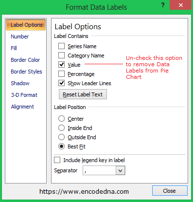
How to display leader lines in pie chart in Excel? - ExtendOffice To display leader lines in pie chart, you just need to check an option then drag the labels out. 1. Click at the chart, and right click to select Format Data Labels from context menu. 2. In the popping Format Data Labels dialog/pane, check Show Leader Lines in the Label Options section. See screenshot: 3. How to add Axis Labels (X & Y) in Excel & Google Sheets How to Add Axis Labels (X&Y) in Excel. Graphs and charts in Excel are a great way to visualize a dataset in a way that is easy to understand. The user should be able to understand every aspect about what the visualization is trying to show right away. As a result, including labels to the X and Y axis is essential so that the user can see what ... How To Match Pie Chart Colors In Excel | Colorpaints.co How To Make A Pie Chart In Excel Add Rich Data Labels The Change The Color Or Style Of A Chart In Office ... How Do I Change The Color Of A Pie Chart In Excel; Share this: Click to share on Twitter (Opens in new window) Click to share on Facebook (Opens in new window) Related.
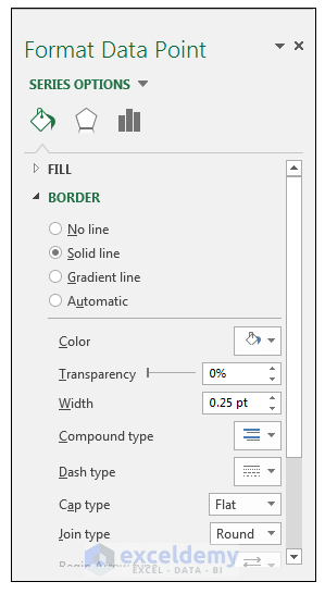
How to add data labels to a pie chart in excel. Pie Chart in Excel - Inserting, Formatting, Filters, Data Labels Click on the Instagram slice of the pie chart to select the instagram. Go to format tab. (optional step) In the Current Selection group, choose data series "hours". This will select all the slices of pie chart. Click on Format Selection Button. As a result, the Format Data Point pane opens. How to Make a PIE Chart in Excel (Easy Step-by-Step Guide) Here are the steps to format the data label from the Design tab: Select the chart. This will make the Design tab available in the ribbon. In the Design tab, click on the Add Chart Element (it's in the Chart Layouts group). Hover the cursor on the Data Labels option. Add or remove data labels in a chart - support.microsoft.com For example, in the pie chart below, without the data labels it would be difficult to tell that coffee was 38% of total sales. Depending on what you want to highlight on a chart, you can add labels to one series, all the series (the whole chart), or one data point. Add data labels. You can add data labels to show the data point values from the ... Change the format of data labels in a chart To get there, after adding your data labels, select the data label to format, and then click Chart Elements > Data Labels > More Options. To go to the appropriate area, click one of the four icons ( Fill & Line, Effects, Size & Properties ( Layout & Properties in Outlook or Word), or Label Options) shown here.
Add a pie chart - support.microsoft.com Click Insert > Insert Pie or Doughnut Chart, and then pick the chart you want. Click the chart and then click the icons next to the chart to add finishing touches: To show, hide, or format things like axis titles or data labels, click Chart Elements . To quickly change the color or style of the chart, use the Chart Styles . Display data point labels outside a pie chart in a paginated report ... Create a pie chart and display the data labels. Open the Properties pane. On the design surface, click on the pie itself to display the Category properties in the Properties pane. Expand the CustomAttributes node. A list of attributes for the pie chart is displayed. Set the PieLabelStyle property to Outside. Set the PieLineColor property to Black. Pie Chart in Excel | How to Create Pie Chart | Step-by-Step ... Large data can be presented by using the Pie Chart in Excel. With the help of each slice bar, we can easily compare one with another. Easy and no need to explain it to the end-user. It is understandable by any means. Disadvantages: Fitting data labels in the case of smaller values is very difficult. It will overlap with other data labels. Inserting Data Label in the Color Legend of a pie chart Small and Medium Business. Public Sector. Internet of Things (IoT) Azure Partner Community. Expand your Azure partner-to-partner network. Microsoft Tech Talks. Bringing IT Pros together through In-Person & Virtual events. MVP Award Program. Find out more about the Microsoft MVP Award Program.
Edit titles or data labels in a chart - support.microsoft.com On a chart, click one time or two times on the data label that you want to link to a corresponding worksheet cell. The first click selects the data labels for the whole data series, and the second click selects the individual data label. Right-click the data label, and then click Format Data Label or Format Data Labels. How to add or move data labels in Excel chart? - ExtendOffice In Excel 2013 or 2016. 1. Click the chart to show the Chart Elements button . 2. Then click the Chart Elements, and check Data Labels, then you can click the arrow to choose an option about the data labels in the sub menu. See screenshot: In Excel 2010 or 2007. 1. click on the chart to show the Layout tab in the Chart Tools group. See ... How to Make a Pie Chart in Excel & Add Rich Data Labels to The Chart! Creating and formatting the Pie Chart. 1) Select the data. 2) Go to Insert> Charts> click on the drop-down arrow next to Pie Chart and under 2-D Pie, select the Pie Chart, shown below. 3) Chang the chart title to Breakdown of Errors Made During the Match, by clicking on it and typing the new title. Possible to add second data label to pie chart? - Excel Help Forum Re: Possible to add second data label to pie chart? Create the composite label in a worksheet column by concatenating the data in other cells and the nextline character, CHR (10). Now, use this composite label column as the source for Rob Bovey's add-in. -- Regards, Tushar Mehta Excel, PowerPoint, and VBA add-ins, tutorials
How to Create a Pie Chart in Excel | Smartsheet
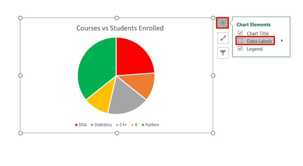
Office: Display Data Labels in a Pie Chart - Tech-Recipes 3. In the Chart window, choose the Pie chart option from the list on the left. Next, choose the type of pie chart you want on the right side. 4. Once the chart is inserted into the document, you will notice that there are no data labels. To fix this problem, select the chart, click the plus button near the chart's bounding box on the right ...
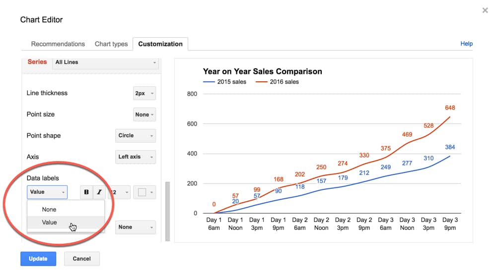
How can I annotate data points in Google Sheets charts? - Ben Collins
Pie of Pie Chart in Excel - Inserting, Customizing - Excel ... Jan 03, 2022 · In the above example, there were a total of 6 data points. The Parent Pie chart represents three of them i.e Facebook, Youtube, and Instagram while the fourth data point named “Other” splits into a subset Pie chart that represents the rest of the three data points i.e Zee, Linkedin, and Hotstar.
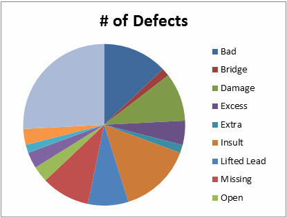
Pie Chart in Excel | Pie Graph | QI Macros Excel Add-in
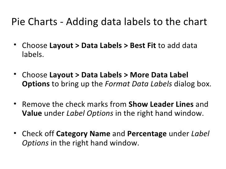
Adding Data Labels to Your Chart (Microsoft Excel) To add data labels in Excel 2013 or Excel 2016, follow these steps: Activate the chart by clicking on it, if necessary. Make sure the Design tab of the ribbon is displayed. (This will appear when the chart is selected.) Click the Add Chart Element drop-down list. Select the Data Labels tool.

Creating a Pie Chart in Excel
How to Make a Pie Chart in Excel - enterprisepc.homelinux.net This wikiHow teaches you how to create a visual representation of your data in Microsoft Excel using a pie chart. Open Microsoft Excel. It resembles a white. ... Add a name to the chart. To do so, click the B1 cell and then type in the chart's name. For example, ...
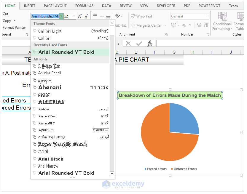
How to Create Excel Pie Charts & Add Rich Data Labels to The Chart!
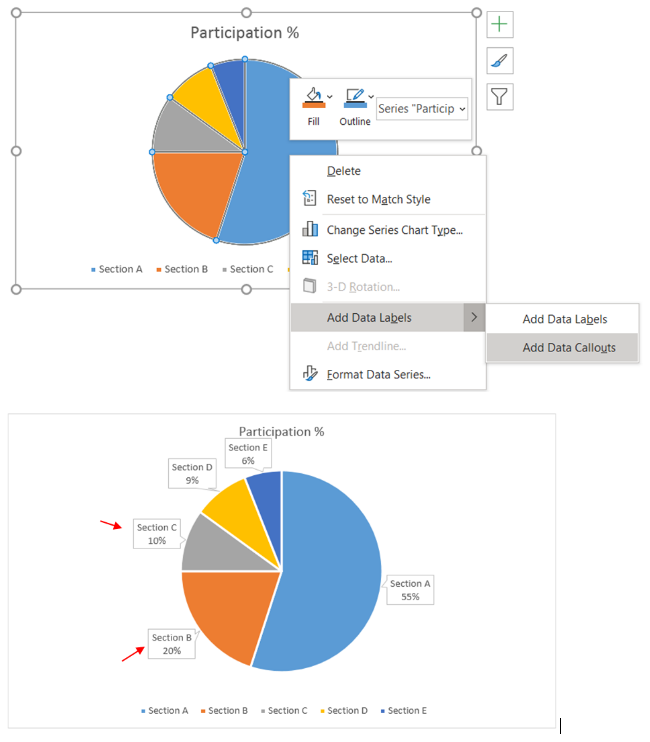
Add data labels and callouts to charts in Excel 365 - EasyTweaks.com The steps that I will share in this guide apply to Excel 2021 / 2019 / 2016. Step #1: After generating the chart in Excel, right-click anywhere within the chart and select Add labels . Note that you can also select the very handy option of Adding data Callouts.
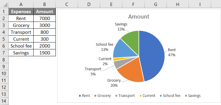
Pie Chart Examples | Types of Pie Charts in Excel with Examples
How to show percentage in pie chart in Excel? - ExtendOffice Select the data you will create a pie chart based on, click Insert > I nsert Pie or Doughnut Chart > Pie. See screenshot: 2. Then a pie chart is created. Right click the pie chart and select Add Data Labels from the context menu. 3. Now the corresponding values are displayed in the pie slices.
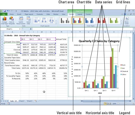
Getting to Know the Parts of an Excel 2010 Chart - dummies
Adding data labels to a pie chart - Excel General - OzGrid Re: Adding data labels to a pie chart. Thanks again, norie. Really appreciate the help. I tried recording a macro while doing it manually (before my first post). But it didn't record anything about labels, much less making them bold.
How to Make a Pie Chart in Excel & Add Rich Data Labels to The Chart!
Excel Pie Chart Examples - TheRescipes.info The Bar of Pie Chart is a built-in chart type in Excel. Pie charts are meant to express a "part to whole" relationship, where all pieces together represent 100%. Pie charts work best to display data with a small number of categories (2-5). The Bar of Pie Chart provides a way to add additional categories to a pie chart without generating a pie ...
How to Create a Pie Chart in Excel using Worksheet Data
How to Create Pie Charts in Excel (In Easy Steps) Select the range A1:D1, hold down CTRL and select the range A3:D3. 6. Create the pie chart (repeat steps 2-3). 7. Click the legend at the bottom and press Delete. 8. Select the pie chart. 9. Click the + button on the right side of the chart and click the check box next to Data Labels.
How to Show Percentage in Pie Chart in Excel? - GeeksforGeeks
How To Match Pie Chart Colors In Excel | Colorpaints.co How To Make A Pie Chart In Excel Add Rich Data Labels The Change The Color Or Style Of A Chart In Office ... How Do I Change The Color Of A Pie Chart In Excel; Share this: Click to share on Twitter (Opens in new window) Click to share on Facebook (Opens in new window) Related.
How to Make a Pie Chart in Excel & Add Rich Data Labels to The Chart!
How to add Axis Labels (X & Y) in Excel & Google Sheets How to Add Axis Labels (X&Y) in Excel. Graphs and charts in Excel are a great way to visualize a dataset in a way that is easy to understand. The user should be able to understand every aspect about what the visualization is trying to show right away. As a result, including labels to the X and Y axis is essential so that the user can see what ...
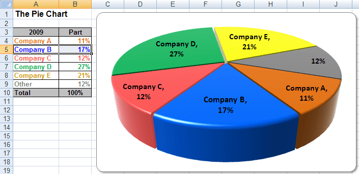
Excel 3-D Pie charts - Microsoft Excel 2010
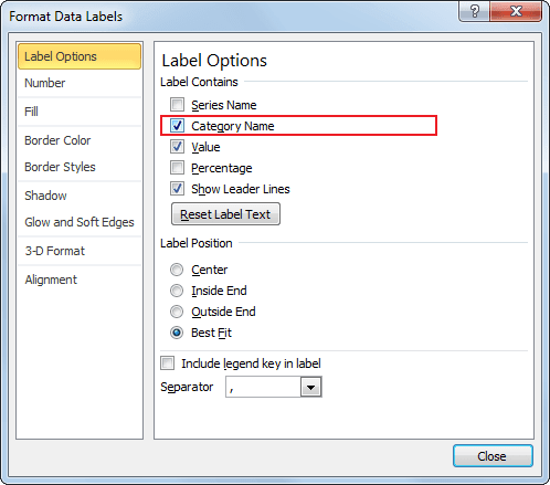
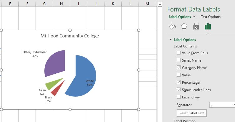
How to display leader lines in pie chart in Excel? - ExtendOffice To display leader lines in pie chart, you just need to check an option then drag the labels out. 1. Click at the chart, and right click to select Format Data Labels from context menu. 2. In the popping Format Data Labels dialog/pane, check Show Leader Lines in the Label Options section. See screenshot: 3.
ExcelSirJi | Excel Data Tips | How to Create Pie Chart in Excel (Complete Tutorial) ExcelSirJi

Breaking down hierarchical data with Treemap and Sunburst charts - Microsoft 365 Blog
4.1 Choosing a Chart Type – Excel For Decision Making
Charts in excel 2007
Excel 3-D Pie Charts

Microsoft Excel Tutorials: Add Data Labels to a Pie Chart
Post a Comment for "40 how to add data labels to a pie chart in excel"