38 pivot table multiple row labels

How to repeat row labels for group in pivot table? - ExtendOffice Except repeating the row labels for the entire pivot table, you can also apply the feature to a specific field in the pivot table only. 1. Firstly, you need to expand the row labels as outline form as above steps shows, and click one row label which you want to repeat in your pivot table. 2. en.wikipedia.org › wiki › Pivot_tablePivot table - Wikipedia Row labels are used to apply a filter to one or more rows that have to be shown in the pivot table. For instance, if the "Salesperson" field is dragged on this area then the other output table constructed will have values from the column "Salesperson", i.e. , one will have a number of rows equal to the number of "Sales Person".

Excel Pivot Table with multiple columns of data and each data … 17.4.2019 · Then I made multiple Pivot Tables, filling the Columns and Values Pivot Table Fields with one Category of each of your categories. This will produce a Pivot Table with 3 rows. The first row will read Column Labels with a filter dropdown. The second row will read all the possible values of the column.

Pivot table multiple row labels

How to make row labels on same line in pivot table in excel #ExcelMaster, #PivotTable, #ExcelHow to make row labels on same line in pivot table in excelHow to show multiple rows in pivot table in excel multiple fields as row labels on the same level in pivot table Excel ... multiple fields as row labels on the same level in pivot table Excel 2016 I am using Excel 2016. I have data that lists product models along with relevant data and also production volumes by month. Part of the relevant data are about 5 common part columns with the part # that applies to each model under the appropriate column. Ranking to a Pivot Table with multiple Row Labels I have a pivot table with multiple Row Labels: Team and Player. I created a second Pts column and used 'Show Values As - Rank Largest to Smallest', but it's not working. It's showing up as '1' for all columns, regardless of whether or not I pick 'Team' or 'Player' as the base field. If I remove 'Team' as a Row Label, however, it works perfectly.

Pivot table multiple row labels. Repeat item labels in a PivotTable - support.microsoft.com Right-click the row or column label you want to repeat, and click Field Settings. Click the Layout & Print tab, and check the Repeat item labels box. Make sure Show item labels in tabular form is selected. When you edit any of the repeated labels, the changes you make are applied to all other cells with the same label. 3 Ways to Display (Multiple Items) Filter Criteria in a Pivot Table The quickest way to see a list of the Multiple Items in the filter is to add a slicer to the pivot table. Select any cell in the pivot table. Select the Analyze/Options tab in the ribbon. Click the Insert Slicer button. Check the box for the field that is in the Filters area with the filter applied to it. Press OK. Pivot table row labels in separate columns • AuditExcel.co.za Our preference is rather that the pivot tables are shown in tabular form (all columns separated and next to each other). You can do this by changing the report format. So when you click in the Pivot Table and click on the DESIGN tab one of the options is the Report Layout. Click on this and change it to Tabular form. How do I show row labels in different columns in PivotTable? Select a cell in the pivot table. On the Ribbon, click the Design tab, and click Report Layout….To show the item labels in every row, for a specific pivot field: Right-click an item in the pivot field. In the Field Settings dialog box, click the Layout & Print tab. Add a check mark to Repeat item labels, then click OK.

Pivot Table Multiple Row Labels? [SOLVED] You can, of course, create a pivot table that sums the values just at the owner level. then, create a second pivot table that sums the values at the Engineer level. If you need to present this data in a contiguous table, you can create a new Excel table and reference to the pivot table values with formulas (=PivotTableSheet!A1) cheers Microsoft MVP excel pivot table - multiple label filters - Stack Overflow 1. As per my comment, you can build a slicer to select/deselect multiple items by holding ctrl whilst selecting with the mouse. Share. Improve this answer. answered Jul 7, 2017 at 11:28. Tim Wilkinson. 3,661 11 32 60. Add a comment. How to Format Excel Pivot Table - Contextures Excel Tips 22.6.2022 · Video: Change Pivot Table Labels. Watch this short video tutorial to see how to make these changes to the pivot table headings and labels. Get the Sample File. No Macros: To experiment with pivot table styles and formatting, download the sample file. The zipped file is in xlsx format, and and does NOT contain any macros. stackoverflow.com › questions › 55735003Excel Pivot Table with multiple columns of data and each data ... Apr 17, 2019 · Then I made multiple Pivot Tables, filling the Columns and Values Pivot Table Fields with one Category of each of your categories. This will produce a Pivot Table with 3 rows. The first row will read Column Labels with a filter dropdown. The second row will read all the possible values of the column.

How to make row labels on same line in pivot table? Make row labels on same line with PivotTable Options You can also go to the PivotTable Options dialog box to set an option to finish this operation. 1. Click any one cell in the pivot table, and right click to choose PivotTable Options, see screenshot: 2. Pivot table row labels side by side - Excel Tutorials You can copy the following table and paste it into your worksheet as Match Destination Formatting. Now, let's create a pivot table ( Insert >> Tables >> Pivot Table) and check all the values in Pivot Table Fields. Fields should look like this. Right-click inside a pivot table and choose PivotTable Options…. Check data as shown on the image below. Pivot table rank example - Exceljet Create a pivot table, and tick "Add data to data model". Add Item field to the rows area. Add Amount as a Value field, and rename to "Sales". Add Amount as a Value field, and rename to "Rank". Set Rank to "largest to smallest with Item as base field. Sort pivot table by Item in descending order. Duplicate Items Appear in Pivot Table - Excel Pivot Tables In Row 2 of the new column, enter the formula =TRIM(C2). Copy the formula down to the last row of data in the source table. If the source data is stored in an Excel Table, the formula should copy down automatically. Refresh the pivot table ; Remove the City field from the pivot table, and add the CityName field to replace it. _____

Discover Pivot Tables – Excel’s most powerful feature and also least known

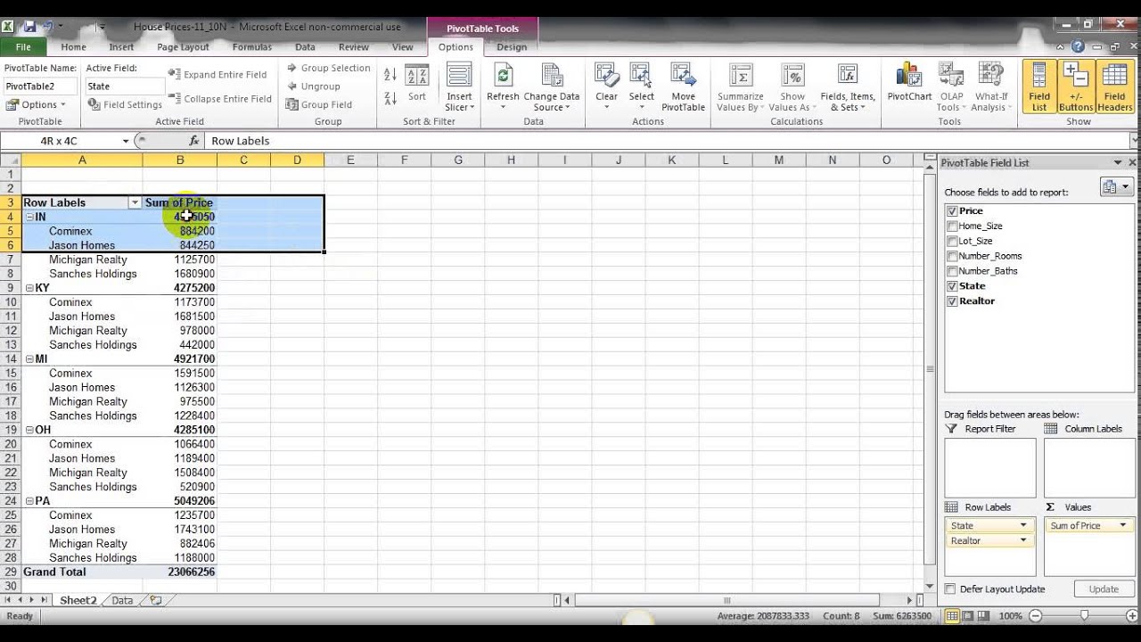
› Add-Rows-to-a-Pivot-TableHow to Add Rows to a Pivot Table: 9 Steps (with Pictures) Feb 15, 2022 · Reorder the field labels in the "Row Labels" section. If you already have a field in the Rows area, adding another row below that will nest the new row within the existing row. [2] X Trustworthy Source Microsoft Support Technical support and product information from Microsoft.

Pivot Table Row Labels In the Same Line - Beat Excel!

How to Filter Multiple Values in Pivot Table - Excel Tutorials When we click OK, we will have only LeBron James selected in our Pivot Table:. Filter with Slicers. Another way to filter multiple values in Pivot Table is to use Slicers.We will create another Pivot Table with the same data. Then we will place player, team, and conference in rows fields and the sum of points, rebounds, assists in the values field.

How to Sort Pivot Table Row Labels, Column Field Labels and Data Values with Excel VBA Macro ...

How to Use Excel Pivot Table Label Filters Right-click a cell in the pivot table, and click PivotTable Options. In the PivotTable Options dialog box, click the Totals & Filters tab In the Filters section, add a check mark to 'Allow multiple filters per field.' Click the OK button, to apply the setting and close the dialog box. Quick Way to Hide or Show Pivot Items

How To Create A Pivot Table With Multiple Columns And Rows | Cabinets Matttroy

How to rename group or row labels in Excel PivotTable? 1. Click at the PivotTable, then click Analyze tab and go to the Active Field textbox. 2. Now in the Active Field textbox, the active field name is displayed, you can change it in the textbox. You can change other Row Labels name by clicking the relative fields in the PivotTable, then rename it in the Active Field textbox.

Multiple Row Filters in Pivot Tables - YouTube

Pivot Table Multiple Row Labels Side By Side | Decorations I Can Make

› excel-pivot-table-formatHow to Format Excel Pivot Table - Contextures Excel Tips Jun 22, 2022 · Video: Change Pivot Table Labels. Watch this short video tutorial to see how to make these changes to the pivot table headings and labels. Get the Sample File. No Macros: To experiment with pivot table styles and formatting, download the sample file. The zipped file is in xlsx format, and and does NOT contain any macros.

Pivot Table Row Labels In the Same Line - Beat Excel!

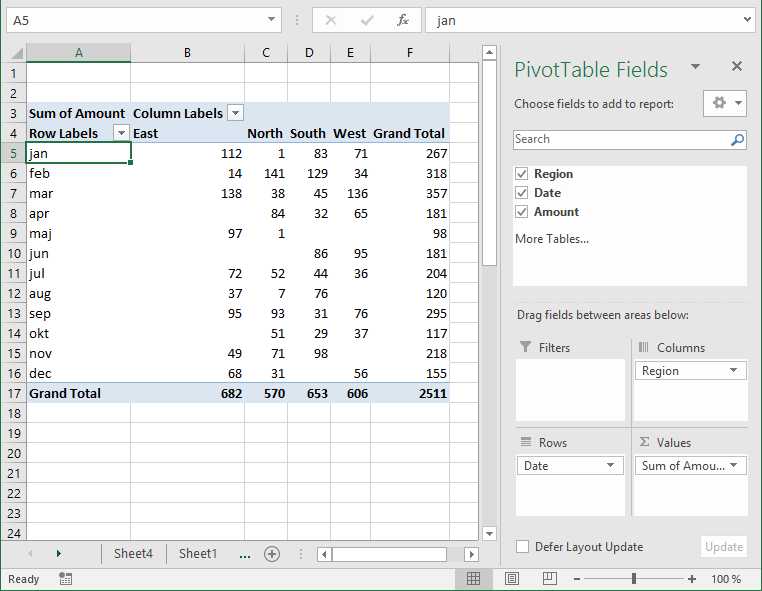
Multi-level Pivot Table in Excel (In Easy Steps) Multiple Row Fields First, insert a pivot table. Next, drag the following fields to the different areas. 1. Category field and Country field to the Rows area. 2. Amount field to the Values area. Below you can find the multi-level pivot table. Multiple Value Fields First, insert a pivot table. Next, drag the following fields to the different areas.

Discover Pivot Tables – Excel’s most powerful feature and also least known

Combining two+ Columns to form one Row label column in Pivot Table Hello, I have multiple sets of data that occur in 2 column increments. The first column is a list of part numbers, the second is their value for that month. I want a pivot table that combines all of the first columns into one master row label of Part numbers and then the values will be listed out in each subsequent column. If a particular month doesn't have a part number in its data, then it ...

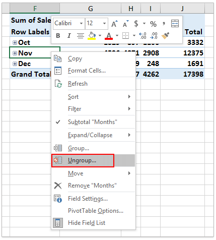
How to ungroup dates in an Excel pivot table?

› pivot-table-tips-and-tricks101 Advanced Pivot Table Tips And Tricks You Need To Know Apr 25, 2022 · As a new pivot table user I LOVE this website – very well written! I do have a unique issue I’m hoping to get assistance with. I have a pivot table built out with multiple rows and columns pertaining to new hire information. My boss likes the option to “drill down” and view the source data.

Pivot Table Row Labels In the Same Line - Beat Excel!

How to add side by side rows in excel pivot table - AnswerTabs To display more pivot table rows side by side, you need to turn on the Classic PivotTable layout and modify Field settings. For example will be used the following table: You have to right-click on pivot table and choose the PivotTable options. Then swich to Display tab and turn on Classic PivotTable layout:

Pivot table row labels in separate columns • AuditExcel.co.za

Multiple row labels on one row in Pivot table | MrExcel Message Board I figured it out - Right click on your pivot table and choose pivot table options/display. Click on "Classic PivotTable layout" Then click on where it is subtotaling your row label and uncheck the subtotal option. D dudeshane0 New Member Joined Oct 23, 2014 Messages 1 Jan 19, 2015 #6 Gerald Higgins said:

How to Show the Percentage of Row Total in the Pivot Table - MS Excel | Excel In Excel

towardsdatascience.com › automate-excel-withAutomate Pivot Table with Python (Create, Filter and Extract) May 22, 2021 · After the Pivot Table is created, wb.Save() will save the Excel file. If this line is not included, the Pivot Table created will be lost. If you are running this script to create Pivot Table in the background or on a scheduled job, you may want to close the Excel file and quit the Excel object by wb.Close(True) and excel.Quit() respectively. In ...

Insert Subtotals to a Pivot Table - Free Microsoft Excel Tutorials

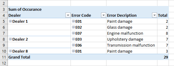
Pivot Table Row Labels In the Same Line - Beat Excel! Then navigate to "Layout & Print" tab and click on "Show item in tabular form" option. Do this procedure also for "Dealer" field and your table will look like this: If you also want dealer names to repeat on each row, reopen "Dealer field settings and check "Repear item labels" option in "Layout & Print" tab.

How To Make Awesome Ranking Charts With Excel Pivot Tables - Moz

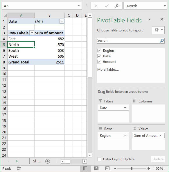
Pivot table - Wikipedia Row labels are used to apply a filter to one or more rows that have to be shown in the pivot table. For instance, if the "Salesperson" field is dragged on this area then the other output table constructed will have values from the column "Salesperson", i.e. , one will have a number of rows equal to the number of "Sales Person".

Naming Columns | CLEARIFY

› xlpivot08Excel Pivot Table Multiple Consolidation Ranges Nov 15, 2021 · Pivot Table from Multiple Consolidation Ranges To open the PivotTable and PivotChart Wizard, select any cell on a worksheet, then press Alt+D, then press P. That shortcut is used because in older versions of Excel, the wizard was listed on the D ata menu, as the P ivotTable and PivotChart Report command.

Abundance Label

38 pivot table multiple row labels

Post a Comment for "38 pivot table multiple row labels"

Menu Halaman Statis