41 multiple data labels excel pie chart

Pie Chart Examples | Types of Pie Charts in Excel ... - EDUCBA PIE Chart can be defined as a circular chart with multiple divisions in it, and each division represents some portion of a total circle or total value. Simply each circle represents the total value of 100 per cent, and each division contributes some per cent to the total. Multiple Data Labels on a Pie Chart - MrExcel Message Board #1 Hello All, So I have a table with 8 rows and 3 columns. This table includes: Column 1 - shipment name Column 2 - shipment cost Column 3 - shipment weight I have created a pie chart from this table, which covers the first two columns. Displayed next to each slice is a label with the shipment name, shipment cost, and percent share of the pie.

How to create a chart in Excel from multiple sheets - Ablebits Nov 05, 2015 · Supposing you have a few worksheets with revenue data for different years and you want to make a chart based on those data to visualize the general trend. 1. Create a chart based on your first sheet. Open your first Excel worksheet, select the data you want to plot in the chart, go to the Insert tab > Charts group, and choose the chart type you ...

Multiple data labels excel pie chart

Plot Multiple Data Sets on the Same Chart in Excel Follow the below steps to implement the same: Step 1: Insert the data in the cells. After insertion, select the rows and columns by dragging the cursor. Step 2: Now click on Insert Tab from the top of the Excel window and then select Insert Line or Area Chart. From the pop-down menu select the first "2-D Line". Change the format of data labels in a chart To get there, after adding your data labels, select the data label to format, and then click Chart Elements > Data Labels > More Options. To go to the appropriate area, click one of the four icons ( Fill & Line, Effects, Size & Properties ( Layout & Properties in Outlook or Word), or Label Options) shown here. Comparison Chart in Excel | Adding Multiple Series Under Same ... This window helps you modify the chart as it allows you to add the series (Y-Values) as well as Category labels (X-Axis) to configure the chart as per your need. Under Legend Entries ( S eries) inside the Select Data Source window, you need to select the sales values for the year 2018 and year 2019.

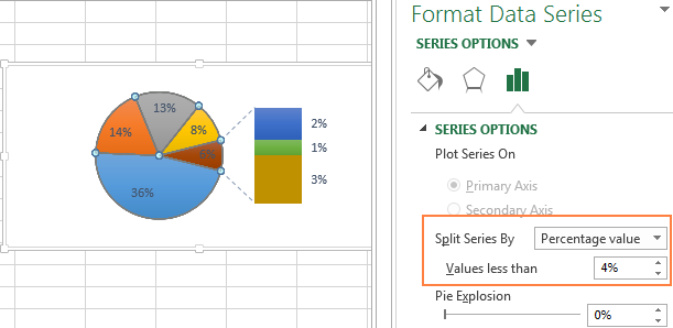
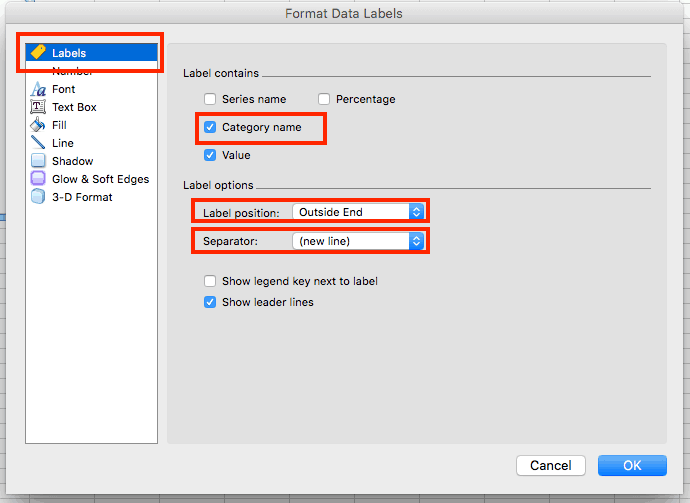
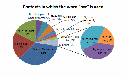
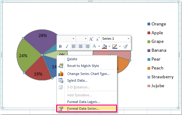
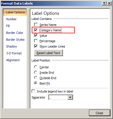
Multiple data labels excel pie chart. How to add two data labels for the same data on a pie chart? Create your pie graph as usual on the "Dashboard" sheet, but remove all labels. Adjust the colors as desired. On your "Calculation sheet, create the text for your percentage label and your ratio label. For example, the first pie chart charts the data 46 and 76. Enter those in A1 and B1. In C1 enter the formula: =A1/SUM (A1,B1) How to display leader lines in pie chart in Excel? To display leader lines in pie chart, you just need to check an option then drag the labels out. 1. Click at the chart, and right click to select Format Data Labels from context menu. 2. In the popping Format Data Labels dialog/pane, check Show Leader Lines in the Label Options section. See screenshot: 3. Close the dialog, now you can see some ... Create a multi-level category chart in Excel - ExtendOffice Create a multi-level category chart in Excel A multi-level category chart can display both the main category and subcategory labels at the same time. When you have values for items that belong to different categories and want to distinguish the values between categories visually, this chart can do you a favor. Pie Charts in Excel - How to Make with Step by Step Examples Task b: Add data labels and data callouts. Step 3: Right-click the pie chart and expand the "add data labels" option. Next, choose "add data labels" again, as shown in the following image. Step 4: The data labels are added to the chart, as shown in the following image.

How to fix wrapped data labels in a pie chart - Sage Intelligence Right click on the data label and select Format Data Labels. 2. Select Text Options > Text Box > and un-select Wrap text in shape. 3. The data labels resize to fit all the text on one line. 4. Alternatively, by double-clicking a data label, the handles can be used to resize the label to wrap words as desired. This can be done on all data labels ... How to Setup a Pie Chart with no Overlapping Labels - Telerik.com Setup a Pie Chart with no overlapping labels. In Design view click on the chart series. The Properties Window will load the selected series properties. Change the DataPointLabelAlignment property to OutsideColumn. Set the value of the DataPointLabelOffset property to a value, providing enough offset from the pie, depending on the chart size (i ... Understanding Excel Chart Data Series, Data Points, and Data ... Sep 19, 2020 · When multiple data series are plotted in one chart, each data series is identified by a unique color or shading pattern. Not all graphs include groups of related data or data series. In column or bar charts, if multiple columns or bars are the same color or have the same picture (in the case of a pictograph ), they comprise a single data series. Pie Chart in Excel | How to Create Pie Chart - EDUCBA Pie Chart in Excel is used for showing the completion or main contribution of different segments out of 100%. It is like each value represents the portion of the Slice from the total complete Pie. For Example, we have 4 values A, B, C and D.

How to Create a Pie Chart in Excel - Smartsheet Enter data into Excel with the desired numerical values at the end of the list. Create a Pie of Pie chart. Double-click the primary chart to open the Format Data Series window. Click Options and adjust the value for Second plot contains the last to match the number of categories you want in the "other" category. Multiple data labels (in separate locations on chart) Re: Multiple data labels (in separate locations on chart) You can do it in a single chart. Create the chart so it has 2 columns of data. At first only the 1 column of data will be displayed. Move that series to the secondary axis. You can now apply different data labels to each series. Attached Files 819208.xlsx‎ (13.8 KB, 264 views) Download Adding data labels to a pie chart - Excel General - OzGrid Excel General. Adding data labels to a pie chart. Laplacian; Feb 24th 2005 ... Adding data labels to a pie chart. Instead of HasDataLabels try ApplyDataLabels, HasDataLabels is not a property of a chart. ... I tried recording multiple macros (create the chart from scratch, modify a created chart, etc.) and still nothing about labels. The macros ... Create two data labels in pie chart? | MrExcel Message Board The boss wants an icon in each data label of a 6-slice pie chart. I can insert the image into the label but it often covers the text and value. Can I create a label for text/value and a second for the image? I can't put any of these values into the pie slice because some of the slices are quite small (<5%) and the data or image are not ...

Microsoft Excel Tutorials: Add Data Labels to a Pie Chart

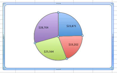
How to Create and Format a Pie Chart in Excel - Lifewire Select the plot area of the pie chart. Right-click the chart. Select Add Data Labels . Select Add Data Labels. In this example, the sales for each cookie is added to the slices of the pie chart. Change Colors When a chart is created in Excel, or whenever an existing chart is selected, two additional tabs are added to the ribbon.

How to make a pie chart in Excel

Select all Data Labels at once - Microsoft Community AFAIK it has never been possible to select all data labels (if there are multiple series) You might be able to use code like this. Sub DL () Dim ocht As Chart Dim ser As Series Dim opt As Point Dim s As Long Dim p As Long Set ocht = ActiveWindow.Selection.ShapeRange (1).Chart For s = 1 To ocht.SeriesCollection.Count

How to Make a Pie Chart in Excel & Add Rich Data Labels to The Chart!

Everything You Need to Know About Pie Chart in Excel Start with selecting your data in Excel. If you include data labels in your selection, Excel will automatically assign them to each column and generate the chart. Go to the INSERT tab in the Ribbon and click on the Pie Chart icon to see the pie chart types. Click on the desired chart to insert. In this example, we're going to be using Pie.

34 How To Label Excel Columns - Labels For You

Creating Pie Chart and Adding/Formatting Data Labels (Excel) Creating Pie Chart and Adding/Formatting Data Labels (Excel) Creating Pie Chart and Adding/Formatting Data Labels (Excel)

How to Create a Pie Chart in Excel | Smartsheet

Formatting data labels and printing pie charts on Excel for Mac 2019 ... Here's a work around I found for printing pie charts. Still can't find a solution for formatting the data labels. 1. When printing a pie chart from Excel for mac 2019, MS instructions are to select the chart only, on the worksheet > file > print. Excel is supposed to print the chart only (not the data ) and automatically fit it onto one page.

Tip : HTML-5 Pie chart long label wrapping in Jasper Studio 6.x & Jasper Server 6.x (OR ...

Pie of Pie Chart in Excel - Inserting, Customizing - Excel ... Jan 03, 2022 · In the above example, there were a total of 6 data points. The Parent Pie chart represents three of them i.e Facebook, Youtube, and Instagram while the fourth data point named “Other” splits into a subset Pie chart that represents the rest of the three data points i.e Zee, Linkedin, and Hotstar.

How to Create a Pie Chart in Excel | Smartsheet

How to Make a Pie Chart in Excel & Add Rich Data Labels to The Chart! Creating and formatting the Pie Chart 1) Select the data. 2) Go to Insert> Charts> click on the drop-down arrow next to Pie Chart and under 2-D Pie, select the Pie Chart, shown below. 3) Chang the chart title to Breakdown of Errors Made During the Match, by clicking on it and typing the new title.

Automatically Group Smaller Slices in Pie Charts to one big Slice

How to Combine or Group Pie Charts in Microsoft Excel Click on the first chart and then hold the Ctrl key as you click on each of the other charts to select them all. Click Format > Group > Group. All pie charts are now combined as one figure. They will move and resize as one image. Choose Different Charts to View your Data

Automatically Group Smaller Slices in Pie Charts to one big Slice | Chandoo.org - Learn ...

Add data labels and callouts to charts in Excel 365 | EasyTweaks.com Step #1: After generating the chart in Excel, right-click anywhere within the chart and select Add labels . Note that you can also select the very handy option of Adding data Callouts. Step #2: When you select the "Add Labels" option, all the different portions of the chart will automatically take on the corresponding values in the table ...

How to Data Labels in a Pie chart in Excel 2010 - YouTube

Excel Pie Chart Multiple Labels | Daily Catalog Click a data label one time to select all data labels in a data series or two times to select just one data label that you want to delete, and then press DELETE. Right-click a data label, and then click Delete. See Also: Excel pie chart add labels Show details Multiple data labels (in separate locations on chart) Preview

Advanced Graphs Using Excel : Gantt Chart in Excel - plot your calender activities

How to add data labels from different column in an Excel chart? This method will introduce a solution to add all data labels from a different column in an Excel chart at the same time. Please do as follows: 1. Right click the data series in the chart, and select Add Data Labels > Add Data Labels from the context menu to add data labels. 2.

How to Make a Pie Chart in Excel & Add Rich Data Labels to The Chart!

How to Show Percentage in Pie Chart in Excel? - GeeksforGeeks Jun 29, 2021 · Select a 2-D pie chart from the drop-down. A pie chart will be built. Select -> Insert -> Doughnut or Pie Chart -> 2-D Pie. Initially, the pie chart will not have any data labels in it. To add data labels, select the chart and then click on the “+” button in the top right corner of the pie chart and check the Data Labels button.

Excel 3-D Pie Charts

Solved: Show multiple data lables on a chart - Power BI I know they can be viewed as tool tips, but this is not sufficient for my needs. Many of my charts are copied to presentations and this added data is necessary for the end users. Solved! Go to Solution. 09-08-2017 12:54 AM. You can set Label Style as All detail labels within the pie chart:

Creating Pie Chart and Adding/Formatting Data Labels (Excel) - YouTube

Add or remove data labels in a chart - support.microsoft.com Click the data series or chart. To label one data point, after clicking the series, click that data point. In the upper right corner, next to the chart, click Add Chart Element > Data Labels. To change the location, click the arrow, and choose an option. If you want to show your data label inside a text bubble shape, click Data Callout.

How to create pie of pie or bar of pie chart in Excel?

Prevent overlapping of data labels in pie chart - Stack Overflow I understand that when the value for one slice of a pie chart is too small, there is bound to have overlap. However, the client insisted on a pie chart with data labels beside each slice (without legends as well) so I'm not sure what other solutions is there to "prevent overlap". Manually moving the labels wouldn't work as the values in the ...

Excel 3-D Pie charts - Microsoft Excel 2007

Comparison Chart in Excel | Adding Multiple Series Under Same ... This window helps you modify the chart as it allows you to add the series (Y-Values) as well as Category labels (X-Axis) to configure the chart as per your need. Under Legend Entries ( S eries) inside the Select Data Source window, you need to select the sales values for the year 2018 and year 2019.

How to Make a Pie Chart in Excel & Add Rich Data Labels to The Chart!

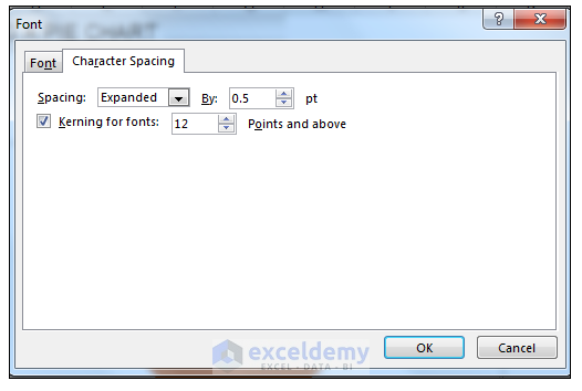
Change the format of data labels in a chart To get there, after adding your data labels, select the data label to format, and then click Chart Elements > Data Labels > More Options. To go to the appropriate area, click one of the four icons ( Fill & Line, Effects, Size & Properties ( Layout & Properties in Outlook or Word), or Label Options) shown here.

Share :