42 excel pie chart with lines to labels

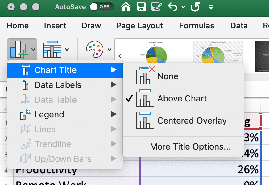
Dynamically Label Excel Chart Series Lines - My Online Training Hub Select the label so the pull handles are displayed, then on the home tab set the font to bold and select the color to match the line. Tip: Select the font color one shade darker than the line to make light colors easier to read. Rinse and repeat steps 3 through 5 for the other series lines. Creating Pie Chart and Adding/Formatting Data Labels (Excel) Creating Pie Chart and Adding/Formatting Data Labels (Excel)

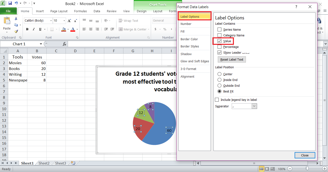
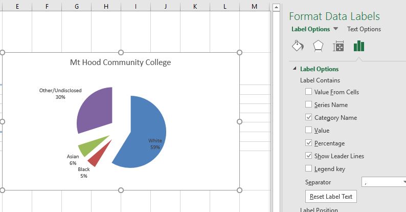
How to display leader lines in pie chart in Excel? To display leader lines in pie chart, you just need to check an option then drag the labels out. 1. Click at the chart, and right click to select Format Data Labels from context menu. 2. In the popping Format Data Labels dialog/pane, check Show Leader Lines in the Label Options section. See screenshot: 3.

Excel pie chart with lines to labels

Pie chart leader lines in excel 2010 - Microsoft Community Replied on September 27, 2013. You the chart selector located in the Current Selection group of the Format contextual tab. Can you see 'Leader Lines 1' ? If yes select that item and use the Format selection button to display format dialog. Check Line Style is set to automatic, or alternative colour if that clashes with the chart area colour. If ... Add data labels and callouts to charts in Excel 365 | EasyTweaks.com Step #1: After generating the chart in Excel, right-click anywhere within the chart and select Add labels . Note that you can also select the very handy option of Adding data Callouts. Step #2: When you select the "Add Labels" option, all the different portions of the chart will automatically take on the corresponding values in the table ... How-to Add Label Leader Lines to an Excel Pie Chart 12 Jun 2013 — . It is that simple. Just make sure it is checked in the label options and then drag and drop an individual data label outside of the pie chart.

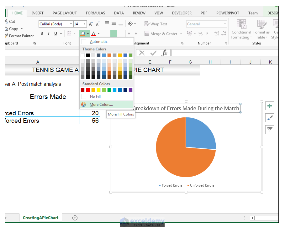
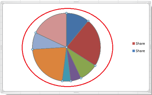
Excel pie chart with lines to labels. Create a Pie Chart in Excel (In Easy Steps) Click the + button on the right side of the chart and click the check box next to Data Labels. 10. Click the paintbrush icon on the right side of the chart and change the color scheme of the pie chart. Result: 11. Right click the pie chart and click Format Data Labels. 12. Check Category Name, uncheck Value, check Percentage and click Center. How to Make a Pie Chart in Excel & Add Rich Data Labels to The Chart! 2) Go to Insert> Charts> click on the drop-down arrow next to Pie Chart and under 2-D Pie, select the Pie Chart, shown below. 3) Chang the chart title to Breakdown of Errors Made During the Match, by clicking on it and typing the new title. How to add leader lines to doughnut chart in Excel? Select data and click Insert > Other Charts > Doughnut. In Excel 2013, click Insert > Insert Pie or Doughnut Chart > Doughnut. 2. Select your original data again, and copy it by pressing Ctrl + C simultaneously, and then click at the inserted doughnut chart, then go to click Home > Paste > Paste Special. See screenshot: 3. Pie Chart in Excel | How to Create Pie Chart - EDUCBA Step 1: Select the data to go to Insert, click on PIE, and select 3-D pie chart. Step 2: Now, it instantly creates the 3-D pie chart for you. Step 3: Right-click on the pie and select Add Data Labels. This will add all the values we are showing on the slices of the pie.

Excel 2010 pie chart data labels in case of "Best Fit" Based on my tested in Excel 2010, the data labels in the "Inside" or "Outside" is based on the data source. If the gap between the data is big, the data labels and leader lines is "outside" the chart. And if the gap between the data is small, the data labels and leader lines is "inside" the chart. Regards, George Zhao TechNet Community Support How to Create Bar of Pie Chart in Excel? Step-by-Step From the Insert tab, select the drop down arrow next to 'Insert Pie or Doughnut Chart'. You should find this in the 'Charts' group. From the dropdown menu that appears, select the Bar of Pie option (under the 2-D Pie category). This will display a Bar of Pie chart that represents your selected data. How to Create and Format a Pie Chart in Excel - Lifewire To add data labels to a pie chart: Select the plot area of the pie chart. Right-click the chart. Select Add Data Labels . Select Add Data Labels. In this example, the sales for each cookie is added to the slices of the pie chart. Change Colors Leader lines for Pie chart are appearing only when the data labels are ... Mar 2, 2017. #2. Leader lines are deemed not necessary in the default position (e.g., outside end). It's only when they are moved, the leader lines are possibly needed because they are further from the point they are labeling. Best fit tries (as best Excel can) to arrange the labels without overlapping. It the wedges are large enough, the ...

Formatting data labels and printing pie charts on Excel for Mac 2019 ... Work around: Select the area of the chart - by selecting the cells behind where the chart is sitting > Print area> Select print area>File > print>then set print perameters (paper size, fit to page etc.) > Print. This worked. 2. When formatting data labels on an extended bar of pie chart: Excel does not allow me to: PIE chart labelling values with reference lines - Tableau null,You can uncheck the allow labels to overlap other marks option below is the snapshot for the same and you can use annotations to recreate the labels for the pie chart as displayed in your snapshot.Note- you will have to manually sort the labels in the view or else they will overlap each other. Move Mark Labels Regards, -AV. How to Create a Pie Chart in Excel | Smartsheet To create a pie chart in Excel 2016, add your data set to a worksheet and highlight it. Then click the Insert tab, and click the dropdown menu next to the image of a pie chart. Select the chart type you want to use and the chosen chart will appear on the worksheet with the data you selected. Office: Display Data Labels in a Pie Chart - Tech-Recipes 3. In the Chart window, choose the Pie chart option from the list on the left. Next, choose the type of pie chart you want on the right side. 4. Once the chart is inserted into the document, you will notice that there are no data labels. To fix this problem, select the chart, click the plus button near the chart's bounding box on the right ...

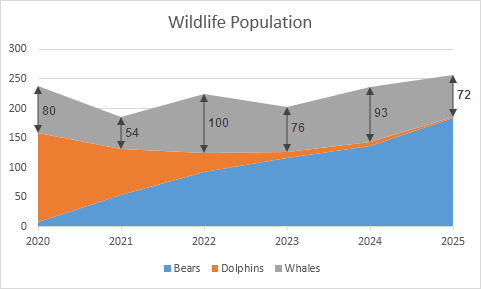
Area Chart in Excel - Easy Excel Tutorial

Formatting Lead Lines on a Chart - MrExcel Message Board When you create a pie chart, you can ask for certain labels, like the name or the amount or the percentage, and when the amounts get too scrunched up, Excel inserts leader lines that drag from the % to the pie piece. I have used the Colo Graphics Exporter to create the jpg file of what it looks like, but I don't know how to post it here.

How to Make a Pie Chart in Excel & Add Rich Data Labels to The Chart!

Pandas scatter plot multiple columns - r23.it The list of Python charts that you can plot using this pandas DataFrame plot function are area, bar, barh, box, density, hexbin, hist, kde, line, pie, scatter. xlsx' sheet_name = 'Data set' writer = pd. Define a grid viewport : a rectangular region on a graphics device. The following is the syntax to create DataFrame in Pandas: pandas.

How to add leader lines to doughnut chart in Excel?

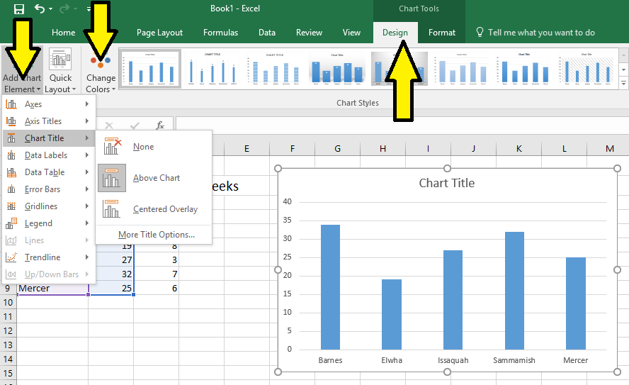
How to Add Gridlines in a Chart in Excel? 2 Easy Ways! To add the gridlines, here are the steps that you need to follow: Click anywhere on the chart. Click on the Chart Elements button (the one with '+' icon). A checklist of chart elements should appear now. Make sure that the checkbox next to 'Gridlines' is checked. This will display the major gridlines on your chart.

How to Create and Format a Pie Chart in Excel

excel - Positioning data labels in pie chart - Stack Overflow Sub tester () Dim se As Series Set se = Totalt.ChartObjects ("Inosa gule").Chart.SeriesCollection ("Grøn pil") se.ApplyDataLabels With se.DataLabels .NumberFormat = "0,0 %" With .Format.Fill .ForeColor.RGB = RGB (255, 255, 255) .Transparency = 0.15 End With .Position = xlLabelPositionCenter End With End Sub

Not All Chart Types Available In Excel For Mac - sgfasr

How to Edit Pie Chart in Excel (All Possible Modifications) How to Edit Pie Chart in Excel 1. Change Chart Color 2. Change Background Color 3. Change Font of Pie Chart 4. Change Chart Border 5. Resize Pie Chart 6. Change Chart Title Position 7. Change Data Labels Position 8. Show Percentage on Data Labels 9. Change Pie Chart's Legend Position 10. Edit Pie Chart Using Switch Row/Column Button 11.

How to Create Histogram in Microsoft Excel? - My Chart Guide

Add Labels with Lines in an Excel Pie Chart (with Easy Steps) 6 days ago — Learn to add labels with lines in an Excel pie chart with some easy steps. You can download an Excel file to practice along with it.

Graphing with Excel - BIOLOGY FOR LIFE

excel - How to not display labels in pie chart that are 0% - Stack Overflow Generate a new column with the following formula: =IF (B2=0,"",A2) Then right click on the labels and choose "Format Data Labels". Check "Value From Cells", choosing the column with the formula and percentage of the Label Options. Under Label Options -> Number -> Category, choose "Custom". Under Format Code, enter the following:

How to Create a Pie Chart in Excel | Smartsheet

How-to Add Label Leader Lines to an Excel Pie Chart - YouTube Step-by-Step Tutorial: how-to create label leader lines that connect pie labels that are outsi...

33 How To Label A Pie Chart In Excel - Labels 2021

Change the format of data labels in a chart To get there, after adding your data labels, select the data label to format, and then click Chart Elements > Data Labels > More Options. To go to the appropriate area, click one of the four icons ( Fill & Line, Effects, Size & Properties ( Layout & Properties in Outlook or Word), or Label Options) shown here.

Excel Charts: Excel Pie Chart With Individual Slice Radius

Add or remove data labels in a chart - support.microsoft.com To label one data point, after clicking the series, click that data point. In the upper right corner, next to the chart, click Add Chart Element > Data Labels. To change the location, click the arrow, and choose an option. If you want to show your data label inside a text bubble shape, click Data Callout.

How to Create a Pie Chart in Excel in 60 Seconds or Less

Excel charts: add title, customize chart axis, legend and data labels To change what is displayed on the data labels in your chart, click the Chart Elements button > Data Labels > More options… This will bring up the Format Data Labels pane on the right of your worksheet. Switch to the Label Options tab, and select the option (s) you want under Label Contains:

How to Create and Label a Pie Chart in Excel 2013 : 8 Steps - Instructables

Adding 2nd Data Label Series to Bar of Pie Chart - Excel Help Forum If you use 2 sets of the same data in the chart you can create 2 pie/bar charts, with one appearing on the secondary axis. Make sure the settings for bar/pie formatting are the same. Add data labels to each series. Format one to show names the other values. Within the pie you may want to delete the name data labels. Attached Files

How to Make a Pie Chart in Excel — Everything You Need to Know

Display data point labels outside a pie chart in a paginated report ... The PieLineColor property defines callout lines for each data point label. To prevent overlapping labels displayed outside a pie chart. Create a pie chart with external labels. On the design surface, right-click outside the pie chart but inside the chart borders and select Chart Area Properties.The Chart AreaProperties dialog box appears. On ...

How-to Add Label Leader Lines to an Excel Pie Chart - Excel Dashboard Templates

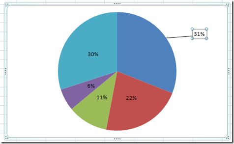
How-to Add Label Leader Lines to an Excel Pie Chart 12 Jun 2013 — . It is that simple. Just make sure it is checked in the label options and then drag and drop an individual data label outside of the pie chart.

Excel Chapter 2 – Business Computers 365

Add data labels and callouts to charts in Excel 365 | EasyTweaks.com Step #1: After generating the chart in Excel, right-click anywhere within the chart and select Add labels . Note that you can also select the very handy option of Adding data Callouts. Step #2: When you select the "Add Labels" option, all the different portions of the chart will automatically take on the corresponding values in the table ...