43 how to add percentage data labels in excel bar chart

Error Bars in Excel (Examples) | How To Add Excel Error Bar? This website or its third-party tools use cookies, which are necessary to its functioning and required to achieve the purposes illustrated in the cookie policy. Column Chart That Displays Percentage Change or Variance 2. Create the Column Chart. The first step is to create the column chart: Select the data in columns C:E, including the header row. On the Insert tab choose the Clustered Column Chart from the Column or Bar Chart drop-down. The chart will be inserted on the sheet and should look like the following screenshot.

How to build a 100% stacked chart with percentages - Exceljet F4 three times will do the job. Now when I copy the formula throughout the table, we get the percentages we need. To add these to the chart, I need select the data labels for each series one at a time, then switch to "value from cells" under label options. Now we have a 100% stacked chart that shows the percentage breakdown in each column.

How to add percentage data labels in excel bar chart

Count and Percentage in a Column Chart - ListenData Steps to show Values and Percentage 1. Select values placed in range B3:C6 and Insert a 2D Clustered Column Chart (Go to Insert Tab >> Column >> 2D Clustered Column Chart). See the image below Insert 2D Clustered Column Chart 2. In cell E3, type =C3*1.15 and paste the formula down till E6 Insert a formula 3. Showing percentages above bars on Excel column graph Update the data labels above the bars to link back directly to other cells Method 2 by step add data-lables right-click the data lable goto the edit bar and type in a refence to a cell (C4 in this example) this changes the data lable from the defulat value (2000) to a linked cell with the 15% Share answered Nov 20, 2013 at 0:30 brettdj How to Change Excel Chart Data Labels to Custom Values? - Chandoo.org First add data labels to the chart (Layout Ribbon > Data Labels) Define the new data label values in a bunch of cells, like this: Now, click on any data label. This will select "all" data labels. Now click once again. At this point excel will select only one data label. Go to Formula bar, press = and point to the cell where the data label ...

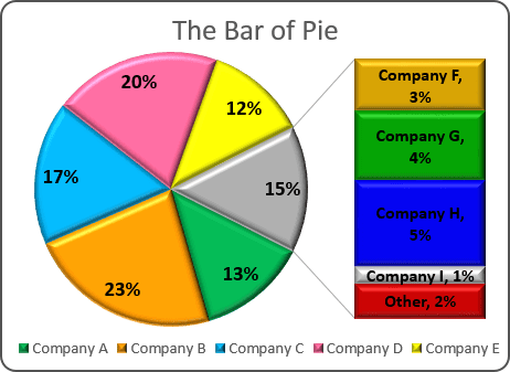
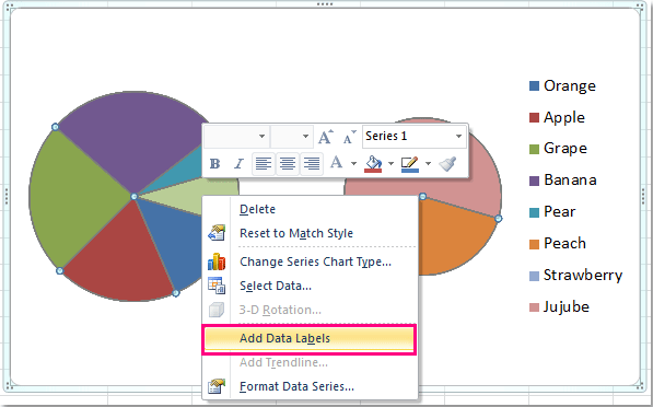
How to add percentage data labels in excel bar chart. How to Create Bar of Pie Chart in Excel? Step-by-Step To be able to see the actual percentage of each portion/ category, adding data labels would be quite helpful. To add and format data labels to portions in your Bar of pie chart, follow the steps below: Click anywhere on the blank area of the chart. You will see three icons appear to the right side of the chart, as shown below: How to Add Percentage Axis to Chart in Excel We will click on the Numbers, then choose Percentage under Category: Our Chart now looks like this: Add Percentage Axis to Chart as Secondary. The above is a fairly easy example as we had only percentages to deal with. Now we want to present all of the data we have on one chart. Luckily, newer versions of Excel are pretty helpful in this regard. Add vertical line to Excel chart: scatter plot, bar and line graph 15/05/2019 · Tips: To change the appearance of the vertical line, right click it, and select Format Data Series in the context menu. This will open the Format Data Series pane, where you can choose the desired dash type, color, etc. For more information, please see How to customize the line in Excel chart.; To add a text label for the line like shown in the image at the beginning of … Add data labels and callouts to charts in Excel 365 - EasyTweaks.com Step #1: After generating the chart in Excel, right-click anywhere within the chart and select Add labels . Note that you can also select the very handy option of Adding data Callouts. Step #2: When you select the "Add Labels" option, all the different portions of the chart will automatically take on the corresponding values in the table ...

How to show percentages in stacked column chart in Excel? - ExtendOffice Add percentages in stacked column chart 1. Select data range you need and click Insert > Column > Stacked Column. See screenshot: 2. Click at the column and then click Design > Switch Row/Column. 3. In Excel 2007, click Layout > Data Labels > Center . In Excel 2013 or the new version, click Design > Add Chart Element > Data Labels > Center. 4. Change the format of data labels in a chart To get there, after adding your data labels, select the data label to format, and then click Chart Elements > Data Labels > More Options. To go to the appropriate area, click one of the four icons ( Fill & Line, Effects, Size & Properties ( Layout & Properties in Outlook or Word), or Label Options) shown here. How to Display Percentage in an Excel Graph (3 Methods) If you want to change the graph axis format from the numbers to percentages, then follow the steps below: First of all, select the cell ranges. Then go to the Insert tab from the main ribbon. From the Charts group, select any one of the graph samples. Now double click on the chart axis that you want to change to percentage. Data label in the graph not showing percentage option. only value ... Data label in the graph not showing percentage option. only value coming. Normally when you put a data label onto a graph, it gives you the option to insert values as numbers or percentages. In the current graph, which I am developing, the percentage option not showing. Enclosed is the screenshot.

How to Show Percentage in Bar Chart in Excel (3 ... - ExcelDemy 3 Methods to Show Percentage in Bar Chart in Excel · =SUM(C5:C9) · =C5/C$10 · ="$"&C5&","&" "&TEXT(C5/C$10,"#%") · =IF(D5>C5, D5-C5,0) · =IF(C5>D5,C5-D5,0) · =MAX(C5: ... Actual vs Budget or Target Chart in Excel - Excel Campus 19/08/2013 · Add the data labels. The variance columns in the data table contain a custom formatting type to display a blank for any zeros: _(* #,##0_);_(* (#,##0);_(* “”_);_(@_) These blanks also display as blanks in the data labels to give the chart a clean look. Otherwise, the variance columns that are not displayed in the chart would still have data labels that display zeros. _ … How to Add Total Data Labels to the Excel Stacked Bar Chart For stacked bar charts, Excel 2010 allows you to add data labels only to the individual components of the stacked bar chart. The basic chart function does not allow you to add a total data label that accounts for the sum of the individual components. Fortunately, creating these labels manually is a fairly simply process. How to Show Percentages in Stacked Column Chart in Excel? Follow the below steps to show percentages in stacked column chart In Excel: Step 1: Open excel and create a data table as below. Step 2: Select the entire data table. Step 3: To create a column chart in excel for your data table. Go to "Insert" >> "Column or Bar Chart" >> Select Stacked Column Chart. Step 4: Add Data labels to the chart.

33 Excel Label Bar Graph - Label Ideas 2020

How to create a chart with both percentage and value in Excel? Select the data range that you want to create a chart but exclude the percentage column, and then click Insert > Insert Column or Bar Chart > 2-D Clustered Column Chart, see screenshot: 2.

How to Show Percentages in Stacked Bar and Column Charts in Excel

Percentage Change Chart – Excel – Automate Excel This tutorial will demonstrate how to create a Percentage Change Chart in all versions of Excel. Percentage Change – Free Template Download Download our free Percentage Template for Excel. Download Now Percentage Change Chart – Excel Starting with your Graph In this example, we’ll start with the graph that shows Revenue for the last 6…

Creating Pie of Pie and Bar of Pie charts - Microsoft Excel 2016

Stacked bar charts showing percentages (excel) - Microsoft Community What you have to do is - select the data range of your raw data and plot the stacked Column Chart and then add data labels. When you add data labels, Excel will add the numbers as data labels. You then have to manually change each label and set a link to the respective % cell in the percentage data range.

How to create pie of pie or bar of pie chart in Excel?

How to add percentage labels to top of bar charts? -Put a label "Year" in your source data -Select all your data -Create the chart bar/line chart -Then select the line part of the chart and right-click -Choose show data labels - then delete the line -finally place the % labels where you want them to be...

How to create pie of pie or bar of pie chart in Excel?

HOW TO CREATE A BAR CHART WITH LABELS ABOVE BAR IN EXCEL - simplexCT In the chart, right-click the Series "Dummy" data series and then, on the shortcut menu, click Add Data Labels. The chart should look like this: 14. In the chart, right-click the Series "Dummy" Data Labels and then, on the short-cut menu, click Format Data Labels. 15.

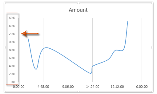
How to format chart axis to percentage in Excel?

How can I show percentage change in a clustered bar chart? Double-click it to open the "Format Data Labels" window. Now select "Value From Cells" (see picture below; made on a Mac, but similar on PC). Then point the range to the list of percentages. If you want to have both the value and the percent change in the label, select both Value From Cells and Values. This will create a label like: -12% 1.729.711

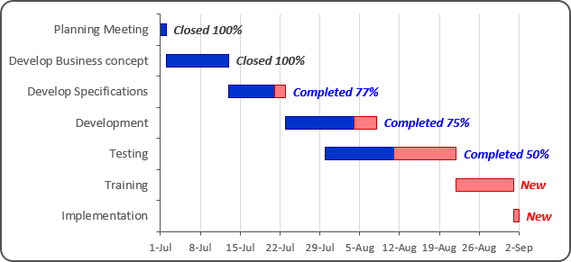
Gantt chart with progress - Microsoft Excel undefined

Add or remove data labels in a chart - support.microsoft.com Click the data series or chart. To label one data point, after clicking the series, click that data point. In the upper right corner, next to the chart, click Add Chart Element > Data Labels. To change the location, click the arrow, and choose an option. If you want to show your data label inside a text bubble shape, click Data Callout.

Share :